Analyze simulation results
This tutorial will use the Fiber from the fiber creation tutorial and simulation results from the simulation and threshold search tutorials. We will analyze the response in transmembrane electric potential (Vm) and gating variables to extracellular stimulation of a fiber over space and time.
Create the fiber and set up simulation
As before, we create a model Fiber, stimulation waveform, extracellular potentials, and a ScaledStim object.
import pyfibers
# Enable logging to see simulation progress and analysis information
pyfibers.enable_logging()
from pyfibers import build_fiber, FiberModel, ScaledStim
import numpy as np
from scipy.interpolate import interp1d
# create fiber model
n_nodes = 25
fiber = build_fiber(
FiberModel.MRG_INTERPOLATION, diameter=10, n_nodes=n_nodes
) # diameter in µm
print(fiber)
# Setup for simulation. Add zeros at the beginning so we get some baseline for visualization
time_step = 0.001 # ms
time_stop = 20 # ms
start, on, off = 0, 0.1, 0.2 # ms
waveform = interp1d(
[start, on, off, time_stop], [0, 1, 0, 0], kind="previous"
) # monophasic rectangular pulse
fiber.potentials = fiber.point_source_potentials(
0, 250, fiber.length / 2, 1, 10
) # x, y, z (µm), i0 (mA), sigma (S/m)
# Create stimulation object
stimulation = ScaledStim(waveform=waveform, dt=time_step, tstop=time_stop)
MRG_INTERPOLATION fiber of diameter 10 µm and length 26936.20 µm
node count: 25, section count: 265.
Fiber is not 3d.
Run simulation
As before, we can simulate the response to a single stimulation pulse.
stimamp = -1.5 # technically unitless, but scales the unit (1 mA) stimulus to 1.5 mA
ap, time = stimulation.run_sim(stimamp, fiber)
print(f'Number of action potentials detected: {ap}')
print(f'Time of last action potential detection: {time} ms')
INFO:pyfibers.stimulation:Running: -1.5
INFO:pyfibers.stimulation:N aps: 1, time 0.379
Number of action potentials detected: 1.0
Time of last action potential detection: 0.379 ms
Before running the simulation, we did not tell the fiber to save any data. Therefore, no transmembrane potential (Vm) or gating variable information was stored. We can confirm this using Python’s hasattr() command.
# checks if the fiber object has the given attribute:
# transmembrane_potentials (vm), gating variables (gating) and transmembrane currents (im)
saved_vm = fiber.vm is not None
print(f"Saved Vm?\n\t{saved_vm}")
saved_gating = fiber.gating is not None
print(f"Saved gating?\n\t{saved_gating}")
saved_im = fiber.im is not None
print(f"Saved Im?\n\t{saved_im}")
Saved Vm?
False
Saved gating?
False
Saved Im?
False
Let’s control the fiber to save the membrane voltage and gating variables and then re-run the simulation. Note that you can record from specific sections of the fiber, record at specific timepoints, or record at a given time step (larger than the simulation time step). For more info, see the Fiber API Documentation. Here, we will proceed with the default usage, which records for all nodes (rather than at every section) at every simulation time step.
fiber.record_vm() # save membrane voltage
fiber.record_gating() # save gating variables
fiber.record_im() # save membrane current
ap, time = stimulation.run_sim(-1.5, fiber)
INFO:pyfibers.stimulation:Running: -1.5
INFO:pyfibers.stimulation:N aps: 1, time 0.379
Now that we have saved membrane voltage and gating variables, let’s take a look at them.
print('Transmembrane potentials (Vm):')
print(fiber.vm)
print('\nGating variables:')
print(fiber.gating)
print('\nTransmembrane currents (Im):')
print(fiber.im)
Transmembrane potentials (Vm):
[Vector[3], Vector[4], Vector[5], Vector[6], Vector[7], Vector[8], Vector[9], Vector[10], Vector[11], Vector[12], Vector[13], Vector[14], Vector[15], Vector[16], Vector[17], Vector[18], Vector[19], Vector[20], Vector[21], Vector[22], Vector[23], Vector[24], Vector[25], Vector[26], Vector[27]]
Gating variables:
{'h': [None, Vector[29], Vector[30], Vector[31], Vector[32], Vector[33], Vector[34], Vector[35], Vector[36], Vector[37], Vector[38], Vector[39], Vector[40], Vector[41], Vector[42], Vector[43], Vector[44], Vector[45], Vector[46], Vector[47], Vector[48], Vector[49], Vector[50], Vector[51], None], 'm': [None, Vector[54], Vector[55], Vector[56], Vector[57], Vector[58], Vector[59], Vector[60], Vector[61], Vector[62], Vector[63], Vector[64], Vector[65], Vector[66], Vector[67], Vector[68], Vector[69], Vector[70], Vector[71], Vector[72], Vector[73], Vector[74], Vector[75], Vector[76], None], 'mp': [None, Vector[79], Vector[80], Vector[81], Vector[82], Vector[83], Vector[84], Vector[85], Vector[86], Vector[87], Vector[88], Vector[89], Vector[90], Vector[91], Vector[92], Vector[93], Vector[94], Vector[95], Vector[96], Vector[97], Vector[98], Vector[99], Vector[100], Vector[101], None], 's': [None, Vector[104], Vector[105], Vector[106], Vector[107], Vector[108], Vector[109], Vector[110], Vector[111], Vector[112], Vector[113], Vector[114], Vector[115], Vector[116], Vector[117], Vector[118], Vector[119], Vector[120], Vector[121], Vector[122], Vector[123], Vector[124], Vector[125], Vector[126], None]}
Transmembrane currents (Im):
[Vector[128], Vector[129], Vector[130], Vector[131], Vector[132], Vector[133], Vector[134], Vector[135], Vector[136], Vector[137], Vector[138], Vector[139], Vector[140], Vector[141], Vector[142], Vector[143], Vector[144], Vector[145], Vector[146], Vector[147], Vector[148], Vector[149], Vector[150], Vector[151], Vector[152]]
We have a NEURON Vector object for each node of the fiber.
Note
By default MRG fibers are created with passive end nodes (see that the first and last values are “None”) to prevent initiation of action potentials at the terminals due to edge-effects. We are simulating the response of a fiber of finite length local to the site of stimulation.
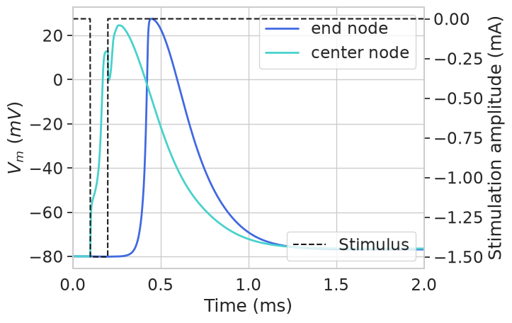
Next, let’s plot the transmembrane voltage for one end compartment and the center compartment to visualize the fiber response to stimulation.
import matplotlib.pyplot as plt
import seaborn as sns
sns.set(font_scale=1.5, style='whitegrid', palette='colorblind')
end_node = 1 # not zero since it was passive and therefore has no data to show!
center_node = fiber.loc_index(0.5)
plt.figure()
plt.plot(
np.array(stimulation.time),
np.array(fiber.vm[end_node]),
label='end node',
color='royalblue',
linewidth=2,
)
plt.plot(
np.array(stimulation.time),
np.array(fiber.vm[center_node]),
label='center node',
color='mediumturquoise',
linewidth=2,
)
plt.legend()
plt.xlabel('Time (ms)')
plt.ylabel('$V_m$ $(mV)$')
ax2 = plt.gca().twinx()
ax2.plot(
np.array(stimulation.time),
stimamp * waveform(stimulation.time),
'k--',
label='Stimulus',
)
ax2.legend(loc=4)
ax2.grid(False)
plt.xlim([0, 2])
plt.ylabel('Stimulation amplitude (mA)')
plt.show()
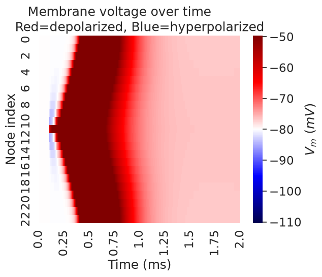
We can plot a heatmap of the voltage across all compartments over time.
import pandas as pd
data = pd.DataFrame(np.array(fiber.vm[1:-1]))
vrest = fiber[0].e_pas
print('Membrane rest voltage:', vrest)
g = sns.heatmap(
data,
cbar_kws={'label': '$V_m$ $(mV)$'},
cmap='seismic',
vmax=np.amax(data.values) + vrest,
vmin=-np.amax(data.values) + vrest,
)
plt.xlim([0, 2000])
plt.ylabel('Node index')
plt.xlabel('Time (ms)')
tick_locs = np.linspace(0, len(np.array(stimulation.time)[:2000]), 9)
labels = [round(np.array(stimulation.time)[int(ind)], 2) for ind in tick_locs]
g.set_xticks(ticks=tick_locs, labels=labels)
plt.title('Membrane voltage over time\
\nRed=depolarized, Blue=hyperpolarized')
Membrane rest voltage: -80.0
Text(0.5, 1.0, 'Membrane voltage over time \nRed=depolarized, Blue=hyperpolarized')
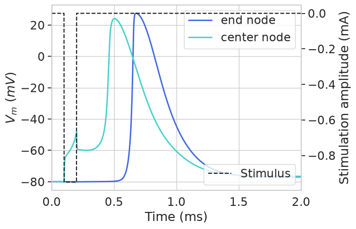
Running a threshold search will also save our variables. Let’s try plotting Vm at threshold.
amp, ap = stimulation.find_threshold(fiber)
print(f'Activation threshold: {amp} mA')
INFO:pyfibers.stimulation:Running: -1
INFO:pyfibers.stimulation:N aps: 1, time 0.437
INFO:pyfibers.stimulation:Running: -0.01
INFO:pyfibers.stimulation:N aps: 0, time None
INFO:pyfibers.stimulation:Search bounds: top=-1, bottom=-0.01
INFO:pyfibers.stimulation:Found AP at 0.437 ms, subsequent runs will exit at 5.437 ms. Change 'exit_t_shift' to modify this.
INFO:pyfibers.stimulation:Beginning bisection search
INFO:pyfibers.stimulation:Search bounds: top=-1, bottom=-0.01
INFO:pyfibers.stimulation:Running: -0.505
INFO:pyfibers.stimulation:N aps: 0, time None
INFO:pyfibers.stimulation:Search bounds: top=-1, bottom=-0.505
INFO:pyfibers.stimulation:Running: -0.7525
INFO:pyfibers.stimulation:N aps: 0, time None
INFO:pyfibers.stimulation:Search bounds: top=-1, bottom=-0.7525
INFO:pyfibers.stimulation:Running: -0.87625
INFO:pyfibers.stimulation:N aps: 0, time None
INFO:pyfibers.stimulation:Search bounds: top=-1, bottom=-0.87625
INFO:pyfibers.stimulation:Running: -0.938125
INFO:pyfibers.stimulation:N aps: 0, time None
INFO:pyfibers.stimulation:Search bounds: top=-1, bottom=-0.938125
INFO:pyfibers.stimulation:Running: -0.969062
INFO:pyfibers.stimulation:N aps: 1, time 0.477
INFO:pyfibers.stimulation:Search bounds: top=-0.969062, bottom=-0.938125
INFO:pyfibers.stimulation:Running: -0.953594
INFO:pyfibers.stimulation:N aps: 1, time 0.548
INFO:pyfibers.stimulation:Search bounds: top=-0.953594, bottom=-0.938125
INFO:pyfibers.stimulation:Running: -0.945859
INFO:pyfibers.stimulation:N aps: 0, time None
INFO:pyfibers.stimulation:Search bounds: top=-0.953594, bottom=-0.945859
INFO:pyfibers.stimulation:Running: -0.949727
INFO:pyfibers.stimulation:N aps: 1, time 0.609
INFO:pyfibers.stimulation:Threshold found at stimamp = -0.949727
INFO:pyfibers.stimulation:Validating threshold...
INFO:pyfibers.stimulation:Running: -0.949727
INFO:pyfibers.stimulation:N aps: 1, time 0.609
Activation threshold: -0.9497265625 mA
# plot vm
plt.figure()
plt.plot(
np.array(stimulation.time),
np.array(fiber.vm[end_node]),
label='end node',
color='royalblue',
linewidth=2,
)
plt.plot(
np.array(stimulation.time),
np.array(fiber.vm[center_node]),
label='center node',
color='mediumturquoise',
linewidth=2,
)
plt.xlim([0, 2])
plt.legend()
plt.xlabel('Time (ms)')
plt.ylabel('$V_m$ $(mV)$')
ax2 = plt.gca().twinx()
ax2.plot(
np.array(stimulation.time),
amp * waveform(stimulation.time),
'k--',
label='Stimulus',
)
ax2.legend(loc=4)
ax2.grid(False)
plt.ylabel('Stimulation amplitude (mA)')
plt.show()
# plot heatmap
data = pd.DataFrame(np.array(fiber.vm[1:-1]))
vrest = fiber[0].e_pas
print('Membrane rest voltage:', vrest)
g = sns.heatmap(
data,
cbar_kws={'label': '$V_m$ $(mV)$'},
cmap='seismic',
vmax=np.amax(data.values) + vrest,
vmin=-np.amax(data.values) + vrest,
)
plt.xlim([0, 2000])
tick_locs = np.linspace(0, len(np.array(stimulation.time)[:2000]), 9)
labels = [round(np.array(stimulation.time)[int(ind)], 2) for ind in tick_locs]
g.set_xticks(ticks=tick_locs, labels=labels)
plt.ylabel('Node index')
plt.xlabel('Time (ms)')
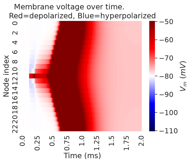
plt.title('Membrane voltage over time. \
\nRed=depolarized, Blue=hyperpolarized')
Membrane rest voltage: -80.0
Text(0.5, 1.0, 'Membrane voltage over time. \nRed=depolarized, Blue=hyperpolarized')
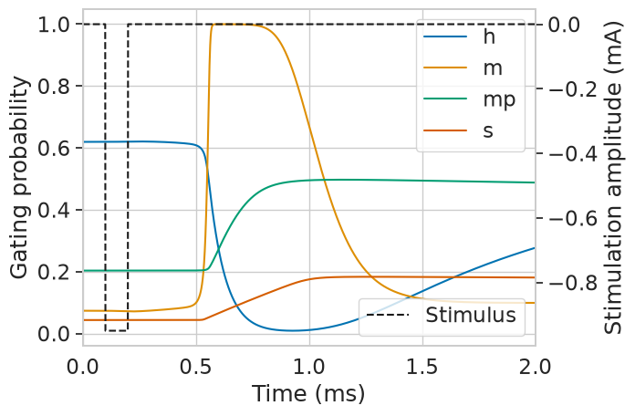
Let’s take a look at the gating variables.
# plot gating variables
plt.figure()
for var in fiber.gating:
plt.plot(np.array(stimulation.time), np.array(fiber.gating[var][6]), label=var)
plt.legend()
plt.xlabel('Time (ms)')
plt.ylabel('Gating probability')
ax2 = plt.gca().twinx()
ax2.plot(
np.array(stimulation.time),
amp * waveform(stimulation.time),
'k--',
label='Stimulus',
)
ax2.legend(loc=4)
ax2.grid(False)
plt.xlim([0, 2])
plt.ylabel('Stimulation amplitude (mA)')
plt.show()
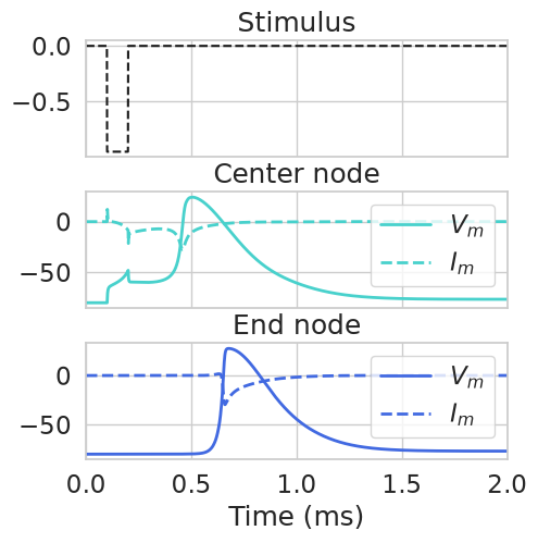
…and the transmembrane currents.
plt.figure()
fig, axs = plt.subplots(3, 1, figsize=(5, 5), sharex=True, gridspec_kw={'hspace': 0.3})
plt.sca(axs[0])
# plot stimulus
plt.plot(
np.array(stimulation.time),
amp * waveform(stimulation.time),
'k--',
label='Stimulus',
)
plt.title('Stimulus')
plt.sca(axs[1])
# plot membrane voltage
plt.plot(
np.array(stimulation.time),
np.array(fiber.vm[center_node]),
color='mediumturquoise',
linewidth=2,
label='$V_m$',
)
# plot im
plt.plot(
np.array(stimulation.time),
np.array(fiber.im[center_node]),
color='mediumturquoise',
linewidth=2,
label='$I_m$',
ls='--',
)
plt.title('Center node')
plt.legend()
plt.sca(axs[2])
# plot end node
plt.plot(
np.array(stimulation.time),
np.array(fiber.vm[end_node]),
color='royalblue',
linewidth=2,
label='$V_m$',
)
plt.plot(
np.array(stimulation.time),
np.array(fiber.im[end_node]),
color='royalblue',
linewidth=2,
label='$I_m$',
ls='--',
)
plt.title('End node')
plt.legend()
plt.xlim([0, 2])
axs[2].set_xlabel('Time (ms)')
plt.show()
<Figure size 640x480 with 0 Axes>
Finally, we can use the data to make videos, which can help visualize how the fiber variables change over time.
from matplotlib.animation import FuncAnimation
# Parameters
skip = 10 # Process every 10th timestep
stop_time = 2 # Stop after 2 milliseconds
# Calculate total number of timesteps available
total_steps = len(fiber.vm[0]) # Assuming each node in fiber.vm is a list or array
n_frames = int(stop_time / (time_step * skip))
ylim = (np.amin(np.array(fiber.vm[1:-1])), np.amax(np.array(fiber.vm[1:-1])))
# Set up the x-axis (node indices or positions)
node_indices = range(1, len(fiber.vm) - 1) # Adjust to match your data
# Set up the figure and axis
fig, ax = plt.subplots()
ax.set_ylim(ylim)
ax.set_xlim(min(node_indices), max(node_indices))
ax.set_xlabel('Node index')
ax.set_ylabel('$V_m$')
(line,) = ax.plot([], [], lw=3, color='mediumturquoise')
title = ax.set_title('')
# Initialize the frame
def init(): # noqa: D103
line.set_data([], [])
title.set_text('')
return line, title
# Update function for animation
def update(frame): # noqa: D103
ind = frame * skip
if ind >= total_steps: # Safety check
return line, title
y_data = [v[ind] for v in fiber.vm[1:-1]]
line.set_data(node_indices, y_data)
title.set_text(f'Time: {ind * time_step:.1f} ms')
return line, title
# Create animation
ani = FuncAnimation(
fig, update, frames=n_frames, init_func=init, blit=True, interval=20
)
# Adjust layout to prevent clipping
plt.tight_layout()
# Display the animation
from IPython.display import HTML
plt.close(fig) # Close the static plot
HTML(ani.to_jshtml())
You can use the same technique to plot videos of other data, such as transmembrane current or gating variables!