Running multiple simulations in parallel
This tutorial will go over the basics of running multiple fiber simulations in parallel. We are often curious about not just a single fiber but an array of fibers with various model types, geometric parameters, and/or electrical parameters. Or, we might want to run the same fiber through multiple simulations. We can leverage parallelism to run multiple simulations simultaneously, each on a separate processor core.
Create a function to parallelize
First, let’s create a function that we can call in parallel. The function should create a Fiber instance and solve for its activation threshold. We will use the fiber model and stimulation parameters from the simulation tutorial. Instead of a single fiber diameter, we will create a function which takes a fiber diameter as an argument, then returns the activation threshold of the fiber.
import pyfibers

# Enable WARNING level logging to avoid noise during parallel simulations
pyfibers.enable_logging(level=pyfibers.logging.WARNING)
def create_and_run_sim(diam=5.7, temp=37):
    """Create a fiber and determine activate threshold.

    :param diam: diameter of fiber (um).
    :param temp: fiber temperature (C)
    :return: activation threshold (mA)
    """
    from pyfibers import build_fiber, FiberModel, ScaledStim
    from scipy.interpolate import interp1d

    # Create fiber object
    fiber = build_fiber(
        FiberModel.MRG_INTERPOLATION, diameter=diam, n_sections=265, temperature=temp
    )

    fiber.potentials = fiber.point_source_potentials(
        0, 250, fiber.length / 2, 1, 10
    )  # x, y, z (µm), i0 (mA), sigma (S/m)

    # Setup for simulation
    time_step = 0.001  # ms
    time_stop = 20  # ms
    waveform = interp1d([0, 0.2, 0.4, time_stop], [1, -1, 0, 0], kind="previous")

    # Create stimulation object
    stimulation = ScaledStim(waveform=waveform, dt=time_step, tstop=time_stop)

    amp, ap = stimulation.find_threshold(fiber)  # Find threshold

    return amp
Parallelization with multiprocess
The multiprocess package provides a way to create and manage multiple processes in Python, similar to how the
threading module handles threads. The Pool object creates a pool of processes which can be used to parallelize our
fiber jobs. See the multiprocess documentation.
Determine available CPUs
Before submitting any jobs, first use the multiprocess package to see the number of cpus available on your machine.
import multiprocess

cpus = multiprocess.cpu_count() - 1
print(cpus)
3
Parallelize fiber jobs for a list of fibers
Now, create an instance of the multiprocess.Pool class. Finally, we can use the Pool.starmap() method in the Pool class to submit our jobs to the process pool. The Pool.starmap() method allows us to pass in a function with multiple arguments to simultaneously submit jobs. For this tutorial, we will demonstrate submitting local parallel jobs to find the activation threshold for a list of fibers, each with a unique diameter.
Note
Note, you must place the Pool.starmap() call inside of an if __name__ == "__main__": statement, as shown below, otherwise your Python code will generate an infinite loop. Besides function definitions, all other functionality you use should be under this statement as well.
from multiprocess import Pool
if __name__ == "__main__":
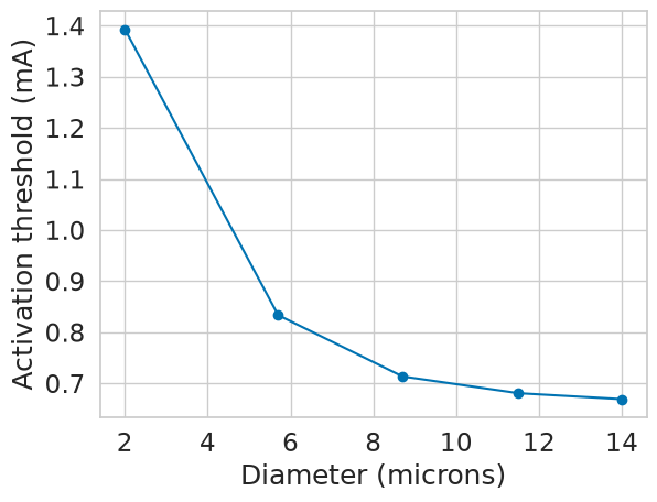
fiber_diams = [2.0, 5.7, 8.7, 11.5, 14.0]
temp = 37
params = [(diam, temp) for diam in fiber_diams]
with Pool(cpus) as p:
results = p.starmap(create_and_run_sim, params)
Let’s plot the activation threshold vs. fiber diameter to see if a relationship between the two exists.
import matplotlib.pyplot as plt
import seaborn as sns
import numpy as np

sns.set(font_scale=1.5, style='whitegrid', palette='colorblind')

plt.figure()
plt.plot(fiber_diams, -np.array(results), marker='o')
plt.xlabel('Diameter (microns)')
plt.ylabel('Activation threshold (mA)')
plt.show()
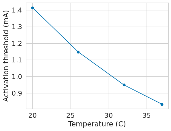
Parallelization is not just limited to running multiple fiber diameters. You could also test the same fiber with different stimulation parameters, or different numbers of sections. Let’s do another example, except this time, let’s vary the number of sections. Again, let’s visualize the data to see if a relationship exists between fiber length and activation threshold.
if __name__ == "__main__":
    diam = 5.7
    temps = [20, 26, 32, 37]
    params = [(diam, temp) for temp in temps]
    with Pool(cpus) as p:
        results = p.starmap(create_and_run_sim, params)
plt.figure()
plt.plot(temps, -np.array(results), marker='o')
plt.xlabel('Temperature (C)')
plt.ylabel('Activation threshold (mA)')
plt.show()