Kilohertz (kHz) Frequency Stimulation Block

This tutorial will use the fiber model created in the simulation tutorial to run a bisection search for the fiber’s block threshold (i.e., the minimum stimulation amplitude needed to stop the progression of a propagating action potential).

Create the fiber and set up simulation

As before, we create a fiber and electrical potentials.

import numpy as np
import matplotlib.pyplot as plt

import scipy.signal as sg
from pyfibers import build_fiber, FiberModel, ScaledStim

# create fiber model
n_nodes = 25
fiber = build_fiber(FiberModel.MRG_INTERPOLATION, diameter=10, n_nodes=n_nodes)

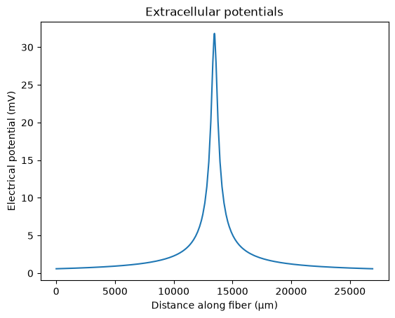
# define unscaled extracellular potentials (in response to a unitary current)
fiber.potentials = fiber.point_source_potentials(0, 250, fiber.length / 2, 1, 10)
plt.plot(fiber.longitudinal_coordinates, fiber.potentials)
plt.xlabel('Distance along fiber (μm)')
plt.ylabel('Electrical potential (mV)')
plt.title('Extracellular potentials')

# turn on saving of transmembrane potential (Vm) so that we can plot it later
fiber.record_vm()

[Vector[1],
 Vector[2],
 Vector[3],
 Vector[4],
 Vector[5],
 Vector[6],
 Vector[7],
 Vector[8],
 Vector[9],
 Vector[10],
 Vector[11],
 Vector[12],
 Vector[13],
 Vector[14],
 Vector[15],
 Vector[16],
 Vector[17],
 Vector[18],
 Vector[19],
 Vector[20],
 Vector[21],
 Vector[22],
 Vector[23],
 Vector[24],
 Vector[25]]

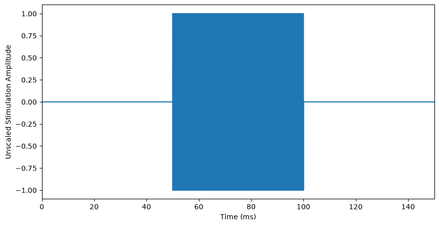
We’ll create a 20 kHz square wave, using a longer time step than in previous tutorials so we have time to observe the fiber’s behavior before, during, and after block. We will set the block signal to only be on from t=50 to t=100 ms. Then we’ll add our waveform to a new ScaledStim instance.

# Setup for simulation
time_step = 0.001  # ms
time_stop = 150  # ms
frequency = 20  # kHz (because our time units are ms)

on, off = 50, 100


# create time vector to make waveform with scipy.signal
# blank out first and last thirds of simulation so we can see block turn on and off
def waveform(t):  # noqa: D
    if t > on and t < off:
        return sg.square(2 * np.pi * frequency * t)
    return 0


# Create stimulation object
blockstim = ScaledStim(waveform=waveform, dt=time_step, tstop=time_stop)

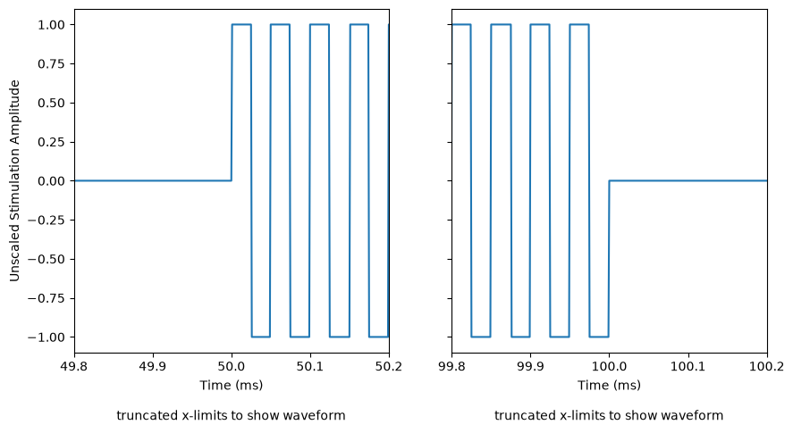
Let’s plot the whole waveform, as well as zoom in to show where it turns on and off.

# whole waveform (cannot see individual pulses)
time_steps = np.arange(0, time_stop, time_step)
plt.plot(time_steps, [waveform(t) for t in time_steps])
plt.xlim([0, 150])
plt.xlabel('Time (ms)')
plt.ylabel('Unscaled Stimulation Amplitude')
plt.gcf().set_size_inches((10, 5))

# create figure to show kilohertz waveform details (turning on and off)
fig, ax = plt.subplots(1, 2, figsize=(10, 5), sharey=True)

# zoom in: kHz turning on
ax[0].plot(time_steps, [waveform(t) for t in time_steps])
ax[0].set_xlim([49.8, 50.2])
ax[0].set_xlabel('Time (ms)\n\ntruncated x-limits to show waveform')
ax[0].set_ylabel('Unscaled Stimulation Amplitude')

# zoom in: kHz turning off
ax[1].plot(time_steps, [waveform(t) for t in time_steps])
ax[1].set_xlim([99.8, 100.2])
ax[1].set_xlabel('Time (ms)\n\ntruncated x-limits to show waveform')

Text(0.5, 0, 'Time (ms)\n\ntruncated x-limits to show waveform')

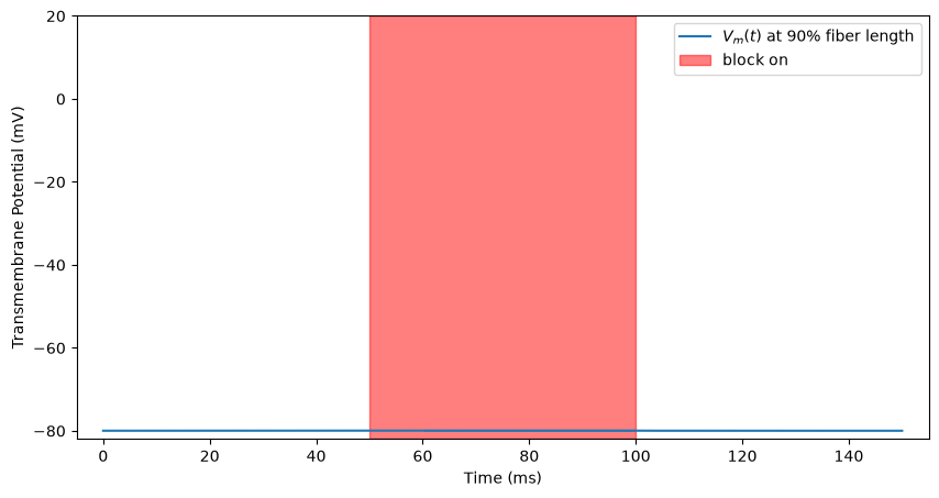
Let’s try stimulating our fiber. We will use a stimulation amplitude low enough that the membrane voltage appears unaffected. This uses the run_sim() method.

ap, time = blockstim.run_sim(-0.5, fiber)

Running: -0.5
	N aps: 0, time None

Let’s create a function to plot our response to the block waveform, which we’ll use going forward. Call it now to plot the fiber response.

def block_plot():
    """Plot the response of a fiber to kHz stimulation."""
    plt.figure(figsize=(10, 5))
    ax = plt.gca()

    ax.plot(
        blockstim.time,
        fiber.vm[fiber.loc_index(0.9)],
        label=r"$V_m(t)$ at 90% fiber length",
    )

    ax.set_xlabel('Time (ms)')
    ax.set_ylabel('Transmembrane Potential (mV)')

    ax.axvspan(50, 100, alpha=0.5, color='red', label='block on')

    # label the synapse activation with vertical black lines
    if fiber.stim:
        for istim_time in np.arange(15, 150, 10):
            label = 'Intracellular stim' if istim_time == 15 else '__'
            ax.axvline(
                x=istim_time, color='black', alpha=0.5, label=label, linestyle='--'
            )

    ax.legend(loc='upper right')
    plt.xlim(-5, 155)


block_plot()
plt.ylim([-82, 20])

(-82.0, 20.0)

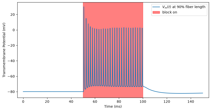
kHz Excitation (below block threshold)

At higher stimulation amplitudes (but still below block threshold), the high frequency stimulation can cause repeated spiking. Let’s turn up the stimulus and watch this happen.

ap, time = blockstim.run_sim(
    -1.5, fiber
)  # NOTE: could happen either above or below threshold
block_plot()

Running: -1.5
	N aps: 27, time 99.386

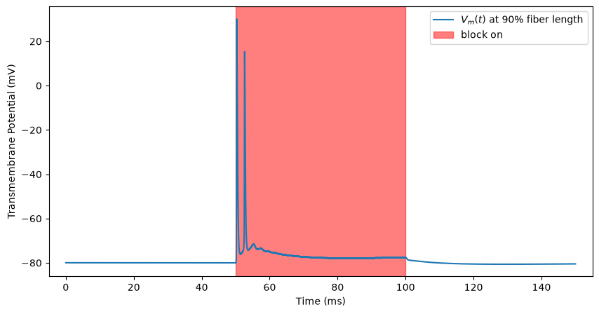
Transmission (with onset response to kHz)

We wanted to stop action potentials, but we are creating many of them! Let’s try turning up the stimulation. You will see an onset response of spiking caused by the stimulation which fades after some time.

ap, time = blockstim.run_sim(-2.5, fiber)
block_plot()

Running: -2.5
	N aps: 2, time 52.566

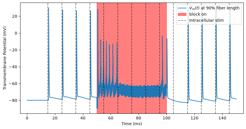
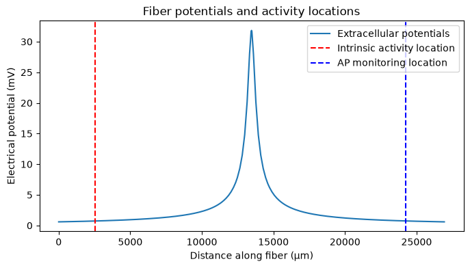
We need to know whether we are truly blocking. We have been recording from one end of the fiber (0.9). Let’s add spiking activity to the other end of the fiber (0.1). At t=15 ms, the activity turns on and a spike occurs every 10 ms. Note that, as we saw in the plot of our extracellular potentials, stimulation is occurring in the center of the fiber (0.5).

We add intrinsic activity using add_intrinsic_activity().

# add intrinsic activity, run with same kHz amplitude as above plot
# loc = 0.1 to avoid erroneous end excitation
fiber.add_intrinsic_activity(loc=0.1, start_time=15, avg_interval=10, num_stims=14)

# plot potentials along fiber, intrinsic activity location, and action potential monitoring location
plt.figure(figsize=(8, 4))
plt.plot(
    fiber.longitudinal_coordinates,
    fiber.potentials[0],
    label='Extracellular potentials',
)
intrinsic_activity_loc = fiber.longitudinal_coordinates[
    fiber.loc_index(0.1, target='sections')
]
monitoring_loc = fiber.longitudinal_coordinates[fiber.loc_index(0.9, target='sections')]
plt.axvline(
    intrinsic_activity_loc,
    color='r',
    linestyle='--',
    label='Intrinsic activity location',
)
plt.axvline(monitoring_loc, color='b', linestyle='--', label='AP monitoring location')
plt.legend()
plt.xlabel('Distance along fiber (μm)')
plt.ylabel('Electrical potential (mV)')
plt.title('Fiber potentials and activity locations')

Text(0.5, 1.0, 'Fiber potentials and activity locations')

We will stimulate using the same amplitude as before.

ap, time = blockstim.run_sim(-2.5, fiber)
block_plot()

Running: -2.5
	N aps: 14, time 145.456

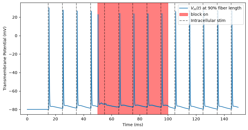
This is called “transmission”, where the action potentials continue unhindered down the axon. The action potential takes time to propagate from one end of the fiber to the other, hence the offset between intracellular stimulation pulses and recorded action potentials.

kHz Block

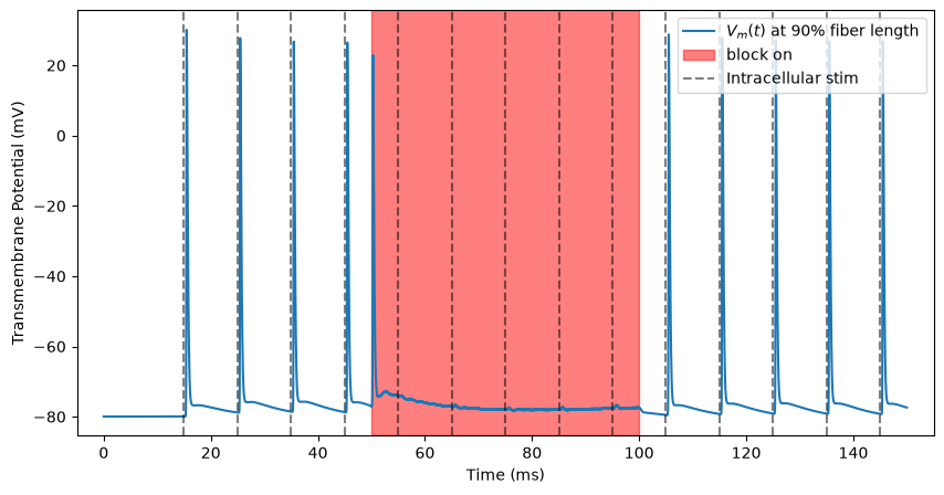
Finally, if we stimulate at an even higher level, we will observe a complete cessation of spike transmission after the block onset response fades.

ap, time = blockstim.run_sim(-3, fiber)
block_plot()

Running: -3
	N aps: 10, time 145.455

Search for kHz block threshold

If we want to determine the block threshold, we can use the find_threshold() method. This method returns the stimulation amplitude at which the fiber begins to block transmission and the number of generated action potentials. We can plot the response of the membrane potential and gating variables at threshold stimulation.

This uses the same algorithm as a search for activation threshold, but here suprathreshold stimulation is considered the absence (rather than the presence) of detected action potentials. Thus, intracellular stimulation is key to determining subthreshold stimulation.

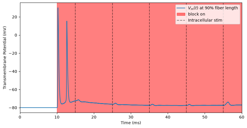
The block_delay parameter defines when the function will start looking for action potentials to evaluate whether transmission is occurring. This should be far enough after block turns on to avoid any false positives due to the onset response. We will also truncate the end of the simulation so that it ends when block turns off.

# Stop simulation when block turns off
blockstim.tstop = 100

# stimamp_top and stimamp_bottom shown to be above and below block threshold, respectively, in previous cells
amp, _ = blockstim.find_threshold(
    fiber,
    condition="block",
    stimamp_top=-3,
    stimamp_bottom=-2,
    exit_t_shift=None,
    block_delay=65,
)
print(f'Block threshold: {amp} mA')
block_plot()

Running: -3
	N aps: 5, time 50.237
Running: -2
	N aps: 10, time 95.554
Search bounds: top=-3, bottom=-2
Beginning bisection search
Search bounds: top=-3, bottom=-2
Running: -2.5
	N aps: 9, time 95.74
Search bounds: top=-3, bottom=-2.5
Running: -2.75
	N aps: 6, time 95.945
Search bounds: top=-3, bottom=-2.75
Running: -2.875
	N aps: 5, time 50.242
Search bounds: top=-2.875, bottom=-2.75
Running: -2.8125
	N aps: 5, time 50.246
Search bounds: top=-2.8125, bottom=-2.75
Running: -2.78125
	N aps: 6, time 96.036
Search bounds: top=-2.8125, bottom=-2.78125
Running: -2.796875
	N aps: 6, time 96.134
Search bounds: top=-2.8125, bottom=-2.796875
Running: -2.804688
	N aps: 6, time 96.237
Threshold found at stimamp = -2.8125
Validating threshold...
Running: -2.8125
	N aps: 5, time 50.246
Block threshold: -2.8125 mA

Re-excitation

It is important to be careful with the upper bound for your block threshold search, as “re-excitation” can occur at suprathreshold stimulation amplitudes. Thus, it is usually safer to set your initial search bounds subthreshold, to avoid any risk of starting with a top bound that causes re-excitation.

blockstim.tstop = 150
ap, time = blockstim.run_sim(
    -250, fiber
)  # NOTE: could happen either above or below threshold
block_plot()

Running: -250
	N aps: 22, time 145.471