Creating fibers using 3D coordinates

Note

This tutorial will use a lot of code explained in the simulation tutorial and the resampling potentials tutorial, so it is recommended to review them before proceeding.

Creating 3D fiber path and potentials

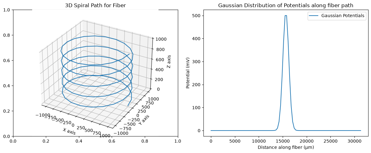
Normally, you might use 3D fiber coordinates alongside potentials that you obtained from an external source (e.g., COMSOL, ANSYS, etc.). For the purpose of this tutorial, we will create a fiber path using a 3D spiral and create potentials using a Gaussian curve. By default, the start of the fiber will be placed at the first coordinate along the path and extend until no more sections can be added. Later in this tutorial, we demonstrate how to shift the fiber to a specific location (typically to achieve some positioning of nodes of Ranvier for myelinated fibers).

# Creating the spiral path for the fiber
import numpy as np
import matplotlib.pyplot as plt

# Define parameters for the spiral
height = 1000  # total height of the spiral
turns = 5  # number of turns in the spiral
radius = 1000  # radius of the spiral
points_per_turn = 20  # points per turn

# Generate the spiral coordinates
t = np.linspace(0, 2 * np.pi * turns, points_per_turn * turns)
x = radius * np.cos(t)
y = radius * np.sin(t)
z = np.linspace(0, height, points_per_turn * turns)

# Combine into a single array for path coordinates
path_coordinates = np.column_stack((x, y, z))

# Plot the generated path to visualize it
fig = plt.figure()
ax = fig.add_subplot(111, projection='3d')
ax.plot(x, y, z)
ax.set_title("3D Spiral Path for Fiber")
ax.set_xlabel("X axis")
ax.set_ylabel("Y axis")
ax.set_zlabel("Z axis")
plt.show()

# Creating potentials along the fiber
# Calculate the length along the fiber
fiber_length = np.sqrt(np.sum(np.diff(path_coordinates, axis=0) ** 2, axis=1)).sum()

# Generate the Gaussian curve of potentials
# Set the mean at the center of the fiber and standard deviation as a fraction of the fiber length
mean = fiber_length / 2
std_dev = fiber_length / 50  # Smaller value gives a narrower peak

# Create an array representing the linear distance along the fiber
linear_distance = np.linspace(0, fiber_length, len(path_coordinates))

# Generate Gaussian distributed potentials
potentials = np.exp(-((linear_distance - mean) ** 2 / (2 * std_dev**2)))

# Normalize potentials for better visualization or use
potentials /= np.max(potentials)

# Scale to a maximum of 500 mV
potentials *= 500

# Plot the Gaussian distribution of potentials along the fiber
plt.figure()
plt.plot(linear_distance, potentials, label='Gaussian Potentials')
plt.xlabel('Distance along fiber (µm)')
plt.ylabel('Potential (mV)')
plt.title('Gaussian Distribution of Potentials along fiber path')
plt.legend()
plt.show()

Resampling 3D potentials

For this tutorial, we will create a fiber model using the MRG model using the same process as the fiber creation tutorial. Instead of specifying the length or number of sections, we provide the coordinates of the 3D fiber path. Since we want a 3D fiber, we must use the function build_fiber_3d() instead.

from pyfibers import FiberModel, build_fiber_3d

fiber = build_fiber_3d(
    FiberModel.MRG_INTERPOLATION, diameter=10, path_coordinates=path_coordinates
)
print(fiber)
print('Fiber is 3D?', fiber.is_3d())

Altering node count from 28 to 27 to enforce odd number.
Altering node count from 28 to 27 to enforce odd number.
MRG_INTERPOLATION fiber of diameter 10 µm and length 29180.80 µm 
	node count: 27, section count: 287. 
	Fiber is 3d.
Fiber is 3D? True

We can either:

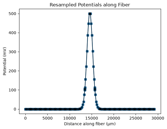
• use the resample_potentials_3d() method of the fiber object to get the potentials at the center of each fiber section. (not recommended)

• or calculate arc lengths and use resample_potentials() to get the potentials. (recommended)

# Using the resample_potentials_3d() method to resample the potentials along the fiber path
fiber.resample_potentials_3d(
    potentials=potentials, potential_coords=path_coordinates, center=True, inplace=True
)

plt.figure()
plt.plot(
    fiber.longitudinal_coordinates,
    fiber.potentials,
    marker='o',
    label='resample_potentials_3d()',
)
plt.xlabel('Distance along fiber (µm)')
plt.ylabel('Potential (mV)')
plt.title('Resampled Potentials along Fiber')

# Calculating arc lengths and using resample_potentials()
arc_lengths = np.concatenate(
    ([0], np.cumsum(np.sqrt(np.sum(np.diff(path_coordinates, axis=0) ** 2, axis=1))))
)
fiber.resample_potentials(
    potentials=potentials, potential_coords=arc_lengths, center=True, inplace=True
)
plt.plot(
    fiber.longitudinal_coordinates,
    fiber.potentials,
    marker='x',
    label='resample_potentials()',
    alpha=0.6,
    color='k',
)

[<matplotlib.lines.Line2D at 0x7f285f8e2c50>]

Simulation

We will use the same simulation setup as before.

import numpy as np
from pyfibers import ScaledStim
from scipy.interpolate import interp1d

# Setup for simulation
time_step = 0.001  # milliseconds
time_stop = 15  # milliseconds
start, on, off = 0, 0.1, 0.2
waveform = interp1d(
    [start, on, off, time_stop], [1, -1, 0, 0], kind="previous"
)  # biphasic rectangular pulse

# Create stimulation object
stimulation = ScaledStim(waveform=waveform, dt=time_step, tstop=time_stop)

and then run a fixed amplitude simulation:

ap, time = stimulation.run_sim(-1.5, fiber)
print(f'Number of action potentials detected: {ap}')
print(f'Time of last action potential detection: {time} ms')

Running: -1.5
	N aps: 1, time 0.301
Number of action potentials detected: 1.0
Time of last action potential detection: 0.301 ms

Creating potentials from a point source

In the previous example, we created potentials using a Gaussian curve. In this example, we will create potentials using a point source. We will use the same fiber path as before, but we will calculate the potentials from a point source near the 3D fiber path.

# Calculate point source potentials at all fiber coordinates
x, y, z = 800, 800, 500  # Point source location
i0 = 1  # Current of the point source
sigma = 1  # Isotropic conductivity
fiber_potentials = fiber.point_source_potentials(x, y, z, i0, sigma, inplace=True)

# Plot
plt.figure()
plt.plot(fiber.longitudinal_coordinates, fiber.potentials, marker='o')
plt.xlabel('Distance along fiber (µm)')
plt.ylabel('Potential (mV)')
plt.title('Fiber potentials from point source')
plt.show()

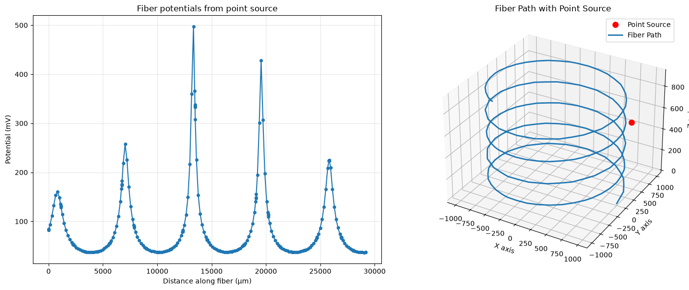
The potentials have several peaks, which would be expected from the location where we placed the point source.

# Plot the fiber with the point source
fig = plt.figure()
ax = fig.add_subplot(111, projection='3d')
ax.plot(x, y, z, 'ro', label='Point Source')
ax.plot(
    fiber.coordinates[:, 0],
    fiber.coordinates[:, 1],
    fiber.coordinates[:, 2],
    label='Fiber Path',
)
ax.set_title('Fiber Path with Point Source')
ax.set_xlabel('X axis')
ax.set_ylabel('Y axis')
ax.set_zlabel('Z axis')
plt.legend()

<matplotlib.legend.Legend at 0x7f285f5c16d0>

Creating fibers with a shift along the 3D path

The prior examples created fibers with the start of the fiber at the beginning of the path. Users may wish to specify a shift along this 3D path to achieve a specific positioning of nodes of Ranvier for myelinated fibers. We can achieve this by specifying the shift along the 3D path using the shift parameter in the build_fiber_3d() function. For this example, we will use a path in 2D space to make it easier to visualize the shift.

# Generate a right angle for fiber path
x = [0, 10000, 10000]
y = [0, 0, 10000]
z = [0, 0, 0]
path_coordinates = np.array([x, y, z]).T

model = FiberModel.MRG_INTERPOLATION
# Create the fiber using the 3D path. Large diameter to space out the nodes
fiber = build_fiber_3d(
    diameter=16,
    fiber_model=model,
    temperature=37,
    path_coordinates=path_coordinates,
    passive_end_nodes=2,
)


def fiber_plot(title):
    """Plot the fiber path and coordinates."""  # noqa: DAR101
    plt.figure()
    # Plot fiber path
    plt.plot(x, y, lw=10, color='gray', alpha=0.3, label='fiber path')
    # Plot fiber coordinates
    plt.plot(
        fiber.coordinates[:, 0],
        fiber.coordinates[:, 1],
        marker='o',
        markersize=5,
        lw=0,
        label='fiber coordinates',
        color='black',
    )
    plt.plot(
        fiber.coordinates[:, 0][::11],
        fiber.coordinates[:, 1][::11],
        marker='o',
        markersize=5,
        lw=0,
        c='r',
        label='nodes',
    )
    plt.title(title)
    plt.gca().set_aspect('equal')
    plt.legend()


fiber_plot('Fiber coordinates (no shift)')

Altering node count from 14 to 13 to enforce odd number.
Altering node count from 14 to 13 to enforce odd number.

We can see that the fiber has been created starting at the beginning of the path. We might want to center the fiber along the path. We can do this by setting center_shift=True.

# Create the fiber using the 3D path, centering the fiber coordinates
fiber = build_fiber_3d(
    diameter=16,
    fiber_model=model,
    temperature=37,
    path_coordinates=path_coordinates,
    passive_end_nodes=2,
    center_shift=True,
    shift_ratio=0.5,
)

fiber_plot('Fiber coordinates (centered)')

Altering node count from 14 to 13 to enforce odd number.
Altering node count from 14 to 13 to enforce odd number.

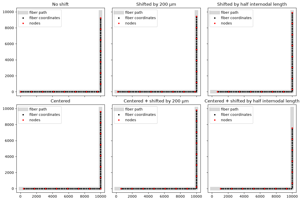
We might want to specify a shift amount along the path. We can do this by setting shift to a value in micrometers, or shift_ratio to a float that represents a proportion of the fiber’s internodal length. Note that distances greater than one internodal length will only be shifted by the remainder (e.g., for a 16 µm diameter fiber with an internodal length of 1600 µm, a shift of 2100 µm will be equivalent to a shift of 500 µm, and a shift_ratio of 1.5 is equivalent to a shift_ratio of 0.5).

# Create the fiber using the 3D path, with no shift
fiber = build_fiber_3d(
    diameter=16,
    fiber_model=model,
    temperature=37,
    path_coordinates=path_coordinates,
    passive_end_nodes=2,
)
fiber_plot('Fiber coordinates (no shift)')

# Create the fiber, shifting by 200 µm
fiber = build_fiber_3d(
    diameter=16,
    fiber_model=model,
    temperature=37,
    path_coordinates=path_coordinates,
    passive_end_nodes=2,
    shift=200,
)
fiber_plot('Fiber coordinates (shifted by 200 µm)')

# Create the fiber, shifting by half the internodal length using shift_ratio
fiber = build_fiber_3d(
    diameter=16,
    fiber_model=model,
    temperature=37,
    path_coordinates=path_coordinates,
    passive_end_nodes=2,
    shift_ratio=0.5,
)
fiber_plot('Fiber coordinates (shifted by half the internodal length)')

Altering node count from 14 to 13 to enforce odd number.
Altering node count from 14 to 13 to enforce odd number.
Altering node count from 14 to 13 to enforce odd number.
Altering node count from 14 to 13 to enforce odd number.
Altering node count from 14 to 13 to enforce odd number.
Altering node count from 14 to 13 to enforce odd number.