Resampling high-resolution potentials

Sometimes you may want to sample potentials agnostic to the final fiber compartment coordinates (e.g., model several fibers along the same trajectory with different diameters, ultrastructure, or membrane mechanisms). This tutorial details how to resample these potentials to match the coordinates of a specific fiber.

Note

This tutorial will use a lot of code explained in the simulation tutorial, so it is recommended to review that before proceeding.

Generate high-resolution potentials

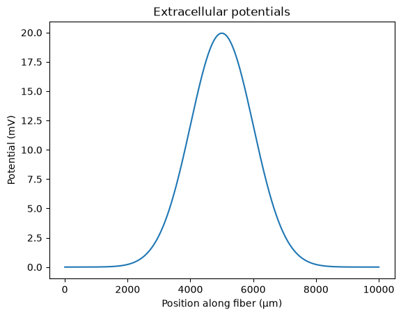
This tutorial provides an example of repurposing electrical potentials that were sampled at high spatial resolution. Users may use external softwares to calculate extracellular potentials (e.g., COMSOL, ANSYS). In this example we will use a gaussian distribution with 5 um spacing between coordinates.

Note

The spacing does not have to be uniform, but the distance between consective points must be suffieciently small to not affect your simulation results. Your coordinates must be one-dimensional arc-lengths along the length of the fiber. If your coordinates are three dimensional, you can use a function such as scipy.spatial.distance.euclidean() to calculate the arc-length between each coordinate, or use a 3D fiber path.

from scipy.stats import norm
import numpy as np
import matplotlib.pyplot as plt

n_coords = 10000

supersampled_potentials = norm.pdf(np.linspace(-1, 1, n_coords), 0, 0.2) * 10
coords = np.cumsum([1] * n_coords)

plt.plot(coords, supersampled_potentials)
plt.title('Extracellular potentials')
plt.xlabel('Position along fiber (\u03bcm)')
plt.ylabel('Potential (mV)')
plt.show()

Create a fiber

For this tutorial, we will create a model Fiber using the MRG model as in the fiber creation tutorial. Instead of specifying the number of coordinates, we will specify the length of our fiber as the length of our super-sampled fiber coordinates.

from pyfibers import build_fiber, FiberModel

fiber_length = np.amax(coords) - np.amin(coords)

fiber = build_fiber(FiberModel.MRG_INTERPOLATION, diameter=10, length=fiber_length)
print(fiber)

Available FiberModel members: ['MRG_DISCRETE', 'MRG_INTERPOLATION', 'PENA', 'RATTAY', 'SCHILD94', 'SCHILD97', 'SMALL_MRG_INTERPOLATION', 'SUNDT', 'SWEENEY', 'THIO_AUTONOMIC', 'THIO_CUTANEOUS', 'TIGERHOLM']
MRG_INTERPOLATION fiber of diameter 10 µm and length 8979.40 µm 
	node count: 9, section count: 89. 
	Fiber is not 3d.

# Helper function for consistent plotting
def plot_fiber_potentials(
    fiber_obj, potentials, title, ax=None, show_full_span=True, use_shifted_coords=False
):
    """Plot fiber potentials with nodes highlighted.

    :param fiber_obj: The fiber object containing coordinates and properties.
    :type fiber_obj: Fiber
    :param potentials: Array of potential values to plot.
    :type potentials: array_like
    :param title: Title for the plot.
    :type title: str
    :param ax: Axes to plot on. If None, creates new figure and axes.
    :type ax: matplotlib.axes.Axes, optional
    :param show_full_span: Whether to show the full potential distribution background.
    :type show_full_span: bool, optional
    :param use_shifted_coords: Whether to use shifted coordinates if available.
    :type use_shifted_coords: bool, optional
    :return: The axes object containing the plot.
    :rtype: matplotlib.axes.Axes
    """
    if ax is None:
        fig, ax = plt.subplots(figsize=(4, 3))

    # Plot the full potential distribution if requested and available
    if (
        show_full_span
        and 'supersampled_potentials' in globals()
        and 'coords' in globals()
    ):
        ax.plot(
            coords,
            supersampled_potentials,
            '-',
            linewidth=1,
            color='lightgray',
            label='potential distribution',
            zorder=-1,
        )

    # Use shifted coordinates if requested and available, otherwise use original coordinates
    if use_shifted_coords and hasattr(fiber_obj, 'shifted_coordinates'):
        plot_coords = fiber_obj.shifted_coordinates
    else:
        plot_coords = fiber_obj.coordinates[:, 2]

    # Plot all sections as dots
    ax.scatter(plot_coords, potentials, s=20, color='black', label='sections')

    # Plot nodes (every 11th point for MRG fibers) as larger red dots
    ax.scatter(plot_coords[::11], potentials[::11], c='red', s=40, label='nodes')

    ax.set_title(title)
    ax.set_xlabel('Position along fiber (μm)')
    ax.set_ylabel('Potential (mV)')
    ax.legend()

    if ax is None:
        plt.show()

    return ax

To obtain potential values at the center of each fiber compartment, we must resample our high-resolution “super sampled” potentials. We can use the resample_potentials() method of the fiber object to do this.

# Compare non-centered vs centered resampling with align_coordinates=True (default)
fig, (ax1, ax2) = plt.subplots(1, 2, figsize=(15, 5))

# Non-centered: align potential coordinates to start at 0
fiber.potentials = fiber.resample_potentials(supersampled_potentials, coords)
plot_fiber_potentials(fiber, fiber.potentials, 'Non-centered', ax=ax1)

# Centered: align midpoints of both coordinate systems
fiber.resample_potentials(supersampled_potentials, coords, center=True, inplace=True)
plot_fiber_potentials(fiber, fiber.potentials, 'Centered', ax=ax2)

plt.tight_layout()
plt.show()

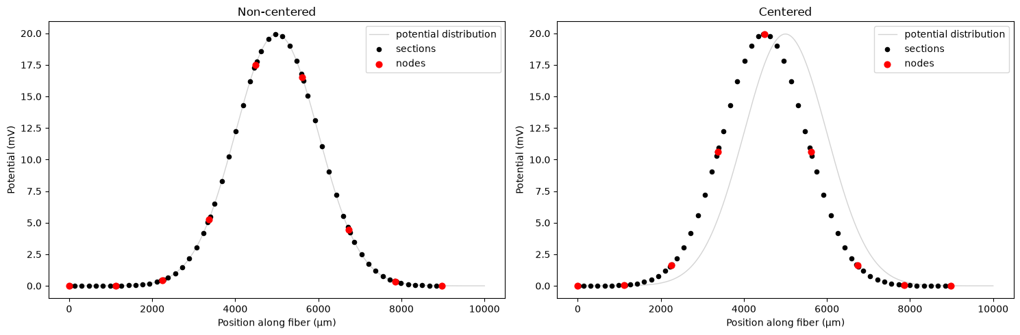
In the left plot, the potential coordinates are aligned to start at 0, so the fiber sits at the edge of the potential distribution. In the right plot, setting center=True samples the fiber potentials from the center of the voltage distribution. Note how the fiber’s longitudinal (arc length) coordinates are unchanged, and so the plotted potentials no longer line up with the original distribution.

Accessing Shifted Coordinates

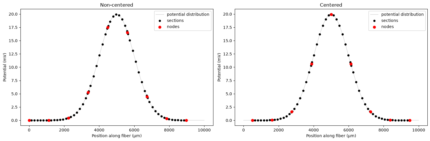
The fiber tracks how much it was shifted during resampling, allowing you to access the effective position of the fiber relative to the potential distribution. Note that this will be overwritten each time you call resample_potentials().

The fiber stores fiber.shifted_coordinates, which is the effective coordinates showing where the fiber sections are positioned after shifting

Why fiber.longitudinal_coordinates stays unchanged: This attribute represents the intrinsic arc-length coordinates based on the fiber’s physical geometry (section lengths and spacing).

Here we use the shifted coordinates to plot the fiber potentials aligned with the distribution we used. Note that all subsequent plots will use the shifted coordinates.

# Using the updated plot_fiber_potentials function with shifted coordinates enabled
fig, (ax1, ax2) = plt.subplots(1, 2, figsize=(15, 5))

# Non-centered
fiber.potentials = fiber.resample_potentials(supersampled_potentials, coords)
plot_fiber_potentials(
    fiber,
    fiber.potentials,
    'Non-centered',
    ax=ax1,
    use_shifted_coords=True,
)

# Centered
fiber.resample_potentials(supersampled_potentials, coords, center=True, inplace=True)
plot_fiber_potentials(
    fiber,
    fiber.potentials,
    'Centered',
    ax=ax2,
    use_shifted_coords=True,
)

plt.tight_layout()
plt.show()

Fiber coordinate shifting during resampling

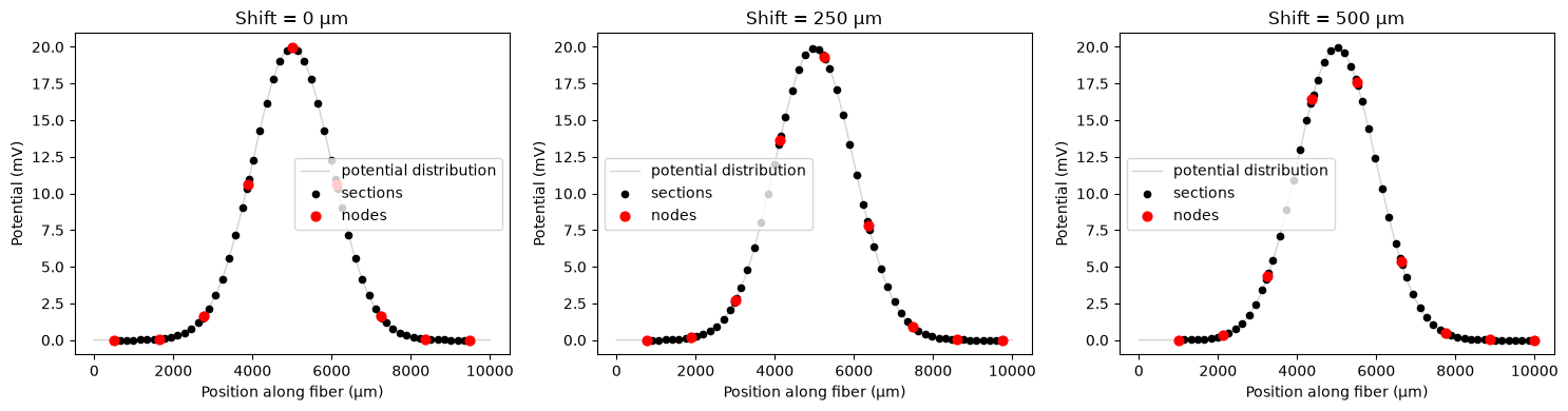
For 1D fibers, you can shift the fiber coordinates during potential resampling to test different fiber positions without recreating the fiber. This is particularly useful when you want to test various alignments with a given potential distribution. Unlike 3D fibers where shifting affects the physical geometry during fiber creation (see the 3D fiber tutorial), 1D fiber shifting is temporary and only affects the potential resampling process.

You can specify shifts using either:

• shift: a shift distance in micrometers (μm), OR

• shift_ratio: a fraction of delta_z (the internodal length)

Note that shifts greater than one internodal length will be reduced using modulus operation (e.g., a shift of 25 μm with a 10 μm internodal length will be equivalent to a 5 μm shift). You can shift with an uncentered fiber as well, but for these examples we will be using a centered fiber.

# Demonstrate basic shifting
print(f"Fiber internodal length (delta_z): {fiber.delta_z:.1f} μm")

# Test different shift values
shift_values = [0, 250, 500]  # μm
fig, axes = plt.subplots(1, 3, figsize=(15, 4))

for i, shift_val in enumerate(shift_values):
    # Apply shift during resampling
    shifted_potentials = fiber.resample_potentials(
        supersampled_potentials,
        coords,
        center=True,
        shift=shift_val,
    )

    plot_fiber_potentials(
        fiber,
        shifted_potentials,
        f'Shift = {shift_val} μm',
        ax=axes[i],
        use_shifted_coords=True,
    )

plt.tight_layout()
plt.show()

Fiber internodal length (delta_z): 1122.3 μm

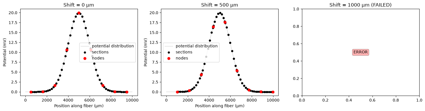
Shifts that are too large and move the fiber outside of the potential range can cause errors. Let’s see this below:

print(f"Current fiber length: {fiber.length:.1f} μm")
print(f"Potential span: {coords[-1] - coords[0]:.1f} μm")
print("\\nTesting shifts with error handling...")

# Test shifts that will likely cause errors
shift_values = [0, 500, 1000]  # μm
fig, axes = plt.subplots(1, 3, figsize=(15, 4))
successful_shifts = []
failed_shifts = []

for i, shift_val in enumerate(shift_values):
    try:
        shifted_potentials = fiber.resample_potentials(
            supersampled_potentials, coords, center=True, shift=shift_val
        )

        plot_fiber_potentials(
            fiber,
            shifted_potentials,
            f'Shift = {shift_val} μm',
            ax=axes[i],
            use_shifted_coords=True,
        )
        successful_shifts.append(shift_val)
        print(f"✓ Shift {shift_val} μm: Success")

    except ValueError as e:
        failed_shifts.append(shift_val)
        axes[i].text(
            0.5,
            0.5,
            'ERROR',
            ha='center',
            va='center',
            transform=axes[i].transAxes,
            bbox={'boxstyle': "round,pad=0.3", 'facecolor': "red", 'alpha': 0.3},
        )
        axes[i].set_title(f'Shift = {shift_val} μm (FAILED)')
        print(f"Shift {shift_val} μm: FAILED")
        print(e)

plt.tight_layout()
plt.show()

print(f"\\nSummary: {len(successful_shifts)} successful, {len(failed_shifts)} failed")
if failed_shifts:
    print("SOLUTION: Create a shorter fiber to accommodate larger shifts")

Current fiber length: 8979.4 μm
Potential span: 9999.0 μm
\nTesting shifts with error handling...
✓ Shift 0 μm: Success
✓ Shift 500 μm: Success
Shift 1000 μm: FAILED
Potential coordinates must span the fiber coordinates. Potential range: [1.000, 10000.000] µm, Target range: [1511.300, 10489.700] µm. Missing coverage: 1510.300 µm at start, 489.700 µm at end. Consider creating a shorter fiber to fit within the potential distribution.
\nSummary: 2 successful, 1 failed
SOLUTION: Create a shorter fiber to accommodate larger shifts

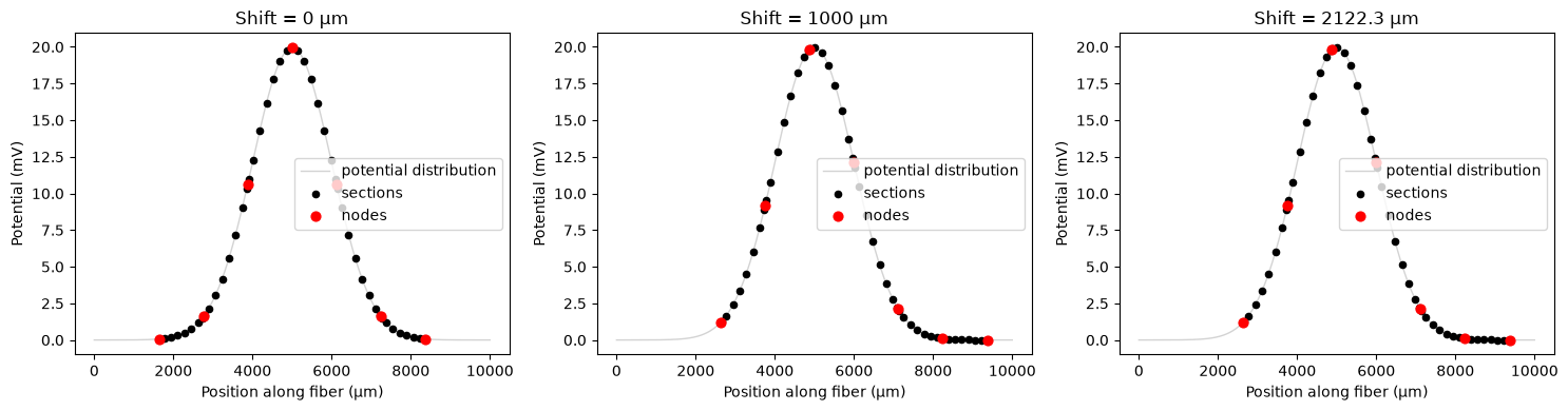
This means we need to create a shorter fiber. Note that any shifts larger than the internodal length will be reduced to the effective shift (since the fiber structure repeats).

# Solution: Rebuild the fiber shorter to accommodate larger shifts
from pyfibers import build_fiber, FiberModel

shorten_by = 2000  # um

fiber_length = np.amax(coords) - np.amin(coords) - shorten_by

fiber = build_fiber(FiberModel.MRG_INTERPOLATION, diameter=10, length=fiber_length)
print(fiber)

# Now test the same shifts with the shorter fiber
# Demonstrate basic shifting
print(f"Fiber internodal length (delta_z): {fiber.delta_z:.1f} μm")

# Test different shift values
shift_values = [
    0,
    1000,
    1000 + fiber.delta_z,
]  # μm, 1000+ fiber.delta_z has the same result as 1000
fig, axes = plt.subplots(1, 3, figsize=(15, 4))

for i, shift_val in enumerate(shift_values):
    # Apply shift during resampling
    shifted_potentials = fiber.resample_potentials(
        supersampled_potentials,
        coords,
        center=True,
        shift=shift_val,
    )

    plot_fiber_potentials(
        fiber,
        shifted_potentials,
        f'Shift = {shift_val} μm',
        ax=axes[i],
        use_shifted_coords=True,
    )

plt.tight_layout()
plt.show()

Altering node count from 8 to 7 to enforce odd number.
MRG_INTERPOLATION fiber of diameter 10 µm and length 6734.80 µm 
	node count: 7, section count: 67. 
	Fiber is not 3d.
Fiber internodal length (delta_z): 1122.3 μm
Note: Requested shift of 2122.300 µm exceeds one internodal length (delta_z = 1122.300 µm). Using equivalent shift of 1000.000 µm instead.

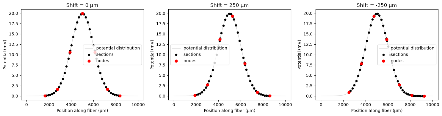
Important: Modulo Behavior and Shift Direction

Critical Understanding: The shifting mechanism uses a modulo operation to ensure that shifts are always applied in the positive direction, regardless of whether you specify a positive or negative shift value. This is because the fiber’s node alignment is the primary concern, not the absolute direction of movement.

What this means:

• Positive shifts (e.g., shift=500): Work as expected, moving the fiber forward

• Negative shifts (e.g., shift=-500): Are converted to equivalent positive shifts using modulo operation

• Large shifts (e.g., shift=2000 with delta_z=1000): Are reduced to equivalent smaller shifts

Why this design choice: The fiber’s electrical properties depend on the alignment of nodes relative to the potential field, not the absolute position. A shift of -500 μm and a shift of +500 μm (when delta_z=1000 μm) result in the same node alignment, so they are treated as equivalent. Fibers are always shifted forward since, by default, they start with one end at z=0.

Example:

# These shifts are equivalent when delta_z = 1000 μm:
shift_1 = 500    # Direct positive shift
shift_2 = -500   # Negative shift → becomes +500 via modulo
shift_3 = 1500   # Large shift → becomes +500 via modulo

This behavior ensures that your fiber positioning is always consistent and predictable, focusing on the electrical alignment rather than geometric movement direction. See the example below, note that the node positionings relative to the potential peak.

# Demonstrate negative shifting
print(f"Fiber internodal length (delta_z): {fiber.delta_z:.1f} μm")

# Test different shift values
shift_values = [0, 250, -250]  # μm
fig, axes = plt.subplots(1, 3, figsize=(15, 4))

for i, shift_val in enumerate(shift_values):
    # Apply shift during resampling
    shifted_potentials = fiber.resample_potentials(
        supersampled_potentials,
        coords,
        center=True,
        shift=shift_val,
    )

    plot_fiber_potentials(
        fiber,
        shifted_potentials,
        f'Shift = {shift_val} μm',
        ax=axes[i],
        use_shifted_coords=True,
    )

plt.tight_layout()
plt.show()

Fiber internodal length (delta_z): 1122.3 μm

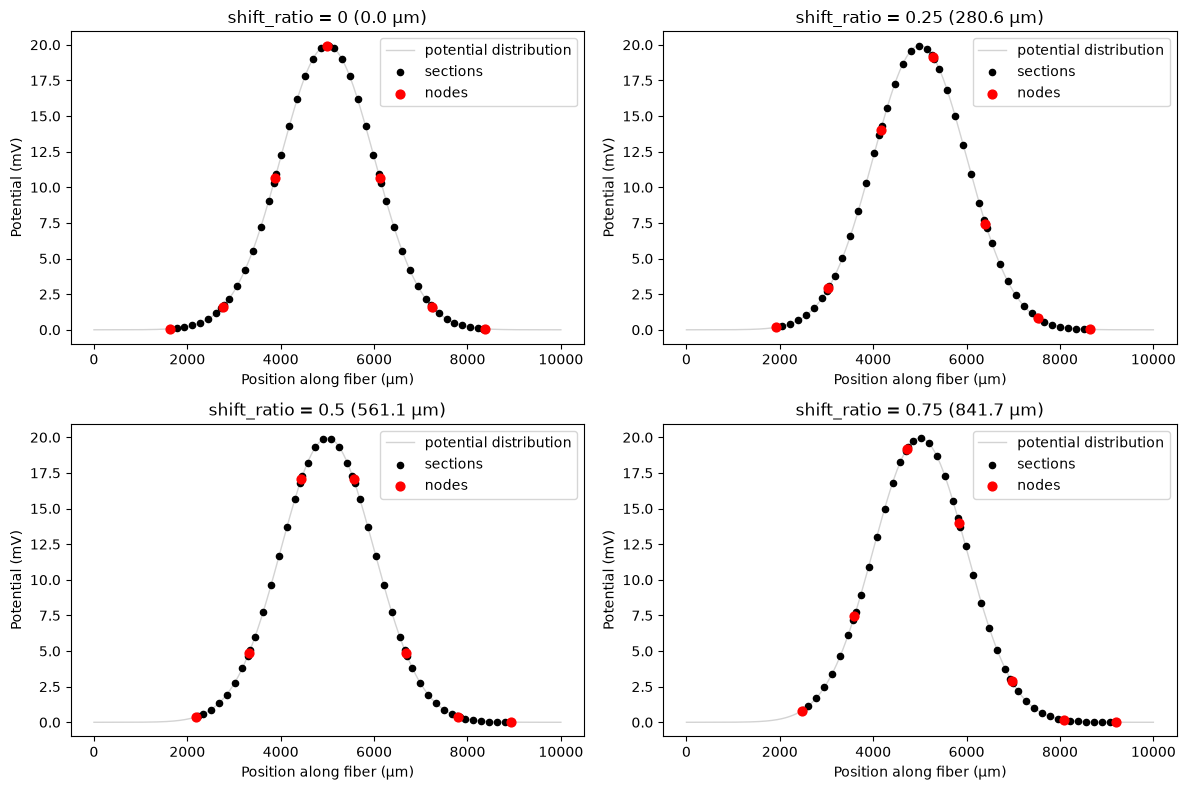
Using shift_ratio for relative positioning

The shift_ratio parameter allows you to specify shifts as a fraction of the internodal length, which is useful for systematic studies across different fiber diameters. A shift_ratio of 0.5 shifts the fiber by half an internodal length, regardless of the actual fiber diameter.

# Demonstrate shift_ratio parameter
shift_ratios = [0, 0.25, 0.5, 0.75]
fig, axes = plt.subplots(2, 2, figsize=(12, 8))
axes = axes.ravel()

for i, shift_ratio in enumerate(shift_ratios):
    # Apply shift_ratio during resampling
    shifted_potentials = fiber.resample_potentials(
        supersampled_potentials, coords, center=True, shift_ratio=shift_ratio
    )

    # Calculate equivalent shift in μm
    equivalent_shift = shift_ratio * fiber.delta_z

    plot_fiber_potentials(
        fiber,
        shifted_potentials,
        f'shift_ratio = {shift_ratio} ({equivalent_shift:.1f} μm)',
        ax=axes[i],
        use_shifted_coords=True,
    )

plt.tight_layout()
plt.show()

Common Use Cases for Resampling and Shifting

The most common use cases for potential resampling and fiber shifting are:

1. Testing different fiber diameters with the same potential distribution

2. Testing different longitudinal alignments (positions) along the potential field

This allows researchers to systematically study how:

• Fiber size affects stimulation thresholds

• Fiber position relative to electrodes affects activation patterns

• Jittering fibers randomly to mimic physiological variability

Simulation

For examples of how to run simulations using the resampled potentials, see the simulation and activation tutorial.