Stimulation from multiple sources

This tutorial will use the simulation results from the simulation tutorial. We will recap that example, and then move on to the case where we have multiple sources. A helpful reference may also be the extracellular potentials documentation.

Create the fiber and set up simulation

As before, we create a fiber using build_fiber(), a stimulation waveform, extracellular potentials, and a stimulation object (an instance of ScaledStim).

import numpy as np
from pyfibers import build_fiber, FiberModel, ScaledStim
from scipy.interpolate import interp1d

# create fiber model
n_sections = 265
fiber = build_fiber(FiberModel.MRG_INTERPOLATION, diameter=10, n_sections=n_sections)
print(fiber)

# Setup for simulation. Add zeros at the beginning so we get some baseline for visualization
time_step = 0.001
time_stop = 20
start, on, off = 0, 0.1, 0.2  # milliseconds
waveform = interp1d(
    [start, on, off, time_stop], [0, 1, 0, 0], kind="previous"
)  # monophasic rectangular pulse

fiber.potentials = fiber.point_source_potentials(0, 250, fiber.length / 2, 1, 10)

# Create stimulation object
stimulation = ScaledStim(waveform=waveform, dt=time_step, tstop=time_stop)

MRG_INTERPOLATION fiber of diameter 10 µm and length 26936.20 µm 
	node count: 25, section count: 265. 
	Fiber is not 3d.

We can then calculate the fiber’s response to stimulation with a certain stimulation amplitude using run_sim().

stimamp = -1.5  # mA
ap, time = stimulation.run_sim(stimamp, fiber)
print(f'Number of action potentials detected: {ap}')
print(f'Time of last action potential detection: {time} ms')

Running: -1.5
	N aps: 1, time 0.379
Number of action potentials detected: 1.0
Time of last action potential detection: 0.379 ms

In many cases, it is desirable to model stimulation of a fiber from multiple sources. There are several ways this can be done:

1. If each source delivers the same waveform, we can simply sum the potentials from each source (using the principle of superposition). In this case, you can weight the potentials if different stimuli deliver different polarities or scaling factors.

2. If each source delivers a different waveform, you must calculate the potentials from each source at runtime. In this case, the fiber must be supplied with multiple potential sets (one for each source), and the ScaledStim instance must be provided with multiple waveforms. You can also use this approach even when each source delivers the same waveform. Under this method, you may either provide a single stimulation amplitude (which is then applied to all sources) or a list of amplitudes (one for each source). Note that for threshold searches, only a single stimulation amplitude is supported.

Superposition of potentials

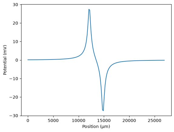
In this example, we will consider the case where we have two sources, each delivering the same waveform. We will calculate the potentials from each source using point_source_potentials(), and sum them to obtain the total potential at each node. This is an example of bipolar stimulation, where one source acts as the anode and the other as the cathode.

fiber.potentials *= 0  # reset potentials
for position, polarity in zip([0.45 * fiber.length, 0.55 * fiber.length], [1, -1]):
    # add the contribution of one source to the potentials
    fiber.potentials += polarity * fiber.point_source_potentials(
        0, 250, position, 1, 10
    )

# plot the potentials
import matplotlib.pyplot as plt

plt.figure()
plt.plot(fiber.longitudinal_coordinates, fiber.potentials[0])
plt.xlabel('Position (μm)')
plt.ylabel('Potential (mV)')
plt.show()

# run simulation
ap, time = stimulation.run_sim(stimamp, fiber)
print(f'Number of action potentials detected: {ap}')
print(f'Time of last action potential detection: {time} ms')

Running: -1.5
	N aps: 1, time 0.416
Number of action potentials detected: 1.0
Time of last action potential detection: 0.416 ms

Sources with different waveforms

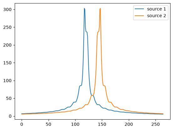
In this example, we consider the case where we have two sources, each delivering a different waveform. In this scenario, you must supply the fiber with multiple potential sets (one for each source) and the ScaledStim instance with multiple waveforms.

potentials = []
# Create potentials from each source
for position in [0.45 * fiber.length, 0.55 * fiber.length]:
    potentials.append(fiber.point_source_potentials(0, 250, position, 1, 1))
fiber.potentials = np.vstack(potentials)
print(fiber.potentials.shape)

plt.figure()
plt.plot(fiber.potentials[0, :], label='source 1')
plt.plot(fiber.potentials[1, :], label='source 2')
plt.legend()

(2, 265)

<matplotlib.legend.Legend at 0x7faf44e8a990>

# Create waveforms and stack them
waveform1 = interp1d(
    [0, 0.05, time_stop], [-1, 0, 0], kind="previous"
)  # monophasic rectangular pulse (cathodic)
waveform2 = interp1d(
    [0, 0.2, time_stop], [1, 0, 0], kind="previous"
)  # monophasic rectangular pulse (longer duration)

# Create instance of :py:class:`~pyfibers.stimulation.ScaledStim`
stimulation = ScaledStim(waveform=[waveform1, waveform2], dt=time_step, tstop=time_stop)

# Turn on saving of gating parameters and Vm before running simulations for thresholds
fiber.record_gating()
fiber.record_vm()

# Run simulation with the same amplitude for all waveforms
ap, time = stimulation.run_sim(-1.5, fiber)
print(f'Number of action potentials detected: {ap}')
print(f'Time of last action potential detection: {time} ms')

# Now, run a simulation with different amplitudes for each waveform
ap, time = stimulation.run_sim([-1.5, 1], fiber)
print(f'Number of action potentials detected: {ap}')
print(f'Time of last action potential detection: {time} ms')

# Finally, run a threshold search (note: only a single stimulation amplitude is supported for threshold searches)
amp, ap = stimulation.find_threshold(fiber, stimamp_top=-3)

Running: -1.5
	N aps: 0, time None
Number of action potentials detected: 0.0
Time of last action potential detection: None ms
Running: [-1.5  1. ]
	N aps: 1, time 0.148
Number of action potentials detected: 1.0
Time of last action potential detection: 0.148 ms
Running: -3
	N aps: 1, time 0.505
Running: -0.01
	N aps: 0, time None
Search bounds: top=-3, bottom=-0.01
Found AP at 0.505 ms, subsequent runs will exit at 5.505 ms. Change 'exit_t_shift' to modify this.
Beginning bisection search
Search bounds: top=-3, bottom=-0.01
Running: -1.505
	N aps: 0, time None
Search bounds: top=-3, bottom=-1.505
Running: -2.2525
	N aps: 1, time 0.449
Search bounds: top=-2.2525, bottom=-1.505
Running: -1.87875
	N aps: 0, time None
Search bounds: top=-2.2525, bottom=-1.87875
Running: -2.065625
	N aps: 0, time None
Search bounds: top=-2.2525, bottom=-2.065625
Running: -2.159062
	N aps: 0, time None
Search bounds: top=-2.2525, bottom=-2.159063
Running: -2.205781
	N aps: 0, time None
Search bounds: top=-2.2525, bottom=-2.205781
Running: -2.229141
	N aps: 1, time 0.454
Search bounds: top=-2.229141, bottom=-2.205781
Running: -2.217461
	N aps: 1, time 0.48
Search bounds: top=-2.217461, bottom=-2.205781
Running: -2.211621
	N aps: 0, time None
Threshold found at stimamp = -2.217461
Validating threshold...
Running: -2.217461
	N aps: 1, time 0.48

import pandas as pd
import seaborn as sns

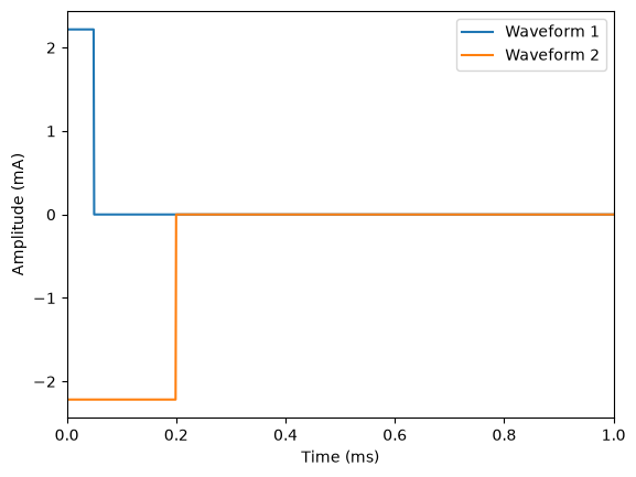
# Plot waveforms
plt.figure()
plt.plot(
    np.array(stimulation.time),
    amp * waveform1(np.array(stimulation.time)),
    label='Waveform 1',
)
plt.plot(
    np.array(stimulation.time),
    amp * waveform2(np.array(stimulation.time)),
    label='Waveform 2',
)
plt.ylabel('Amplitude (mA)')
plt.xlabel('Time (ms)')
plt.legend()
plt.xlim([0, 1])

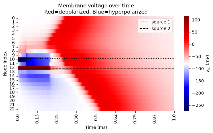
# Plot heatmap of membrane voltage (Vm)
data = pd.DataFrame(np.array(fiber.vm[1:-1]))
vrest = fiber[0].e_pas
print('Membrane rest voltage:', vrest)
plt.figure()
g = sns.heatmap(
    data,
    cbar_kws={'label': '$V_m$ $(mV)$'},
    cmap='seismic',
    vmax=np.amax(data.values) + vrest,
    vmin=-np.amax(data.values) + vrest,
)
plt.ylabel('Node index')
plt.xlabel('Time (ms)')
tick_locs = np.linspace(0, len(np.array(stimulation.time)[:1000]), 9)
labels = [round(np.array(stimulation.time)[int(ind)], 2) for ind in tick_locs]
g.set_xticks(ticks=tick_locs, labels=labels)
plt.title('Membrane voltage over time\nRed=depolarized, Blue=hyperpolarized')
plt.xlim([0, 1000])
# label source locations
for loc, ls, label in zip([0.45, 0.55], [':', '--'], ['source 1', 'source 2']):
    location = loc * (len(fiber)) - 1
    plt.axhline(location, color='black', linestyle=ls, label=label)
plt.legend()
plt.gcf().set_size_inches(8.15, 4)

Membrane rest voltage: -80.0