Recording single fiber action potentials

This tutorial will use the model Fiber from the fiber creation tutorial to run a simulation of fiber activity and simulate a recording electrode placed nearby.

Create the fiber and run simulation

As before, we create Fiber, waveform, potentials and ScaledStim object.

import numpy as np
from pyfibers import build_fiber, FiberModel, ScaledStim
from scipy.interpolate import interp1d

# create fiber model
n_nodes = 25
fiber = build_fiber(FiberModel.MRG_INTERPOLATION, diameter=10, n_nodes=n_nodes)

# Setup for simulation
time_step = 0.001
time_stop = 10
start, on, off = 0, 0.1, 0.2
waveform = interp1d(
    [start, on, off, time_stop], [0, 1, 0, 0], kind="previous"
)  # biphasic rectangular pulse

fiber.potentials = fiber.point_source_potentials(0, 250, fiber.length / 2, 1, 10)

# Create stimulation object
stimulation = ScaledStim(waveform=waveform, dt=time_step, tstop=time_stop)

As before, we can simulate the response to a single stimulation pulse:

fiber.record_vm()
ap, time = stimulation.run_sim(-1.5, fiber)
print(f'Number of action potentials detected: {ap}')
print(f'Time of last action potential detection: {time} ms')

Running: -1.5
	N aps: 1, time 0.379
Number of action potentials detected: 1.0
Time of last action potential detection: 0.379 ms

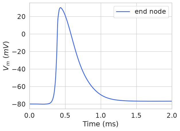
Then we can plot the membrane potential at the end of the fiber:

import matplotlib.pyplot as plt
import seaborn as sns

sns.set(font_scale=1.5, style='whitegrid', palette='colorblind')

plt.figure()
plt.plot(
    np.array(stimulation.time)[:2000],
    list(fiber.vm[fiber.loc_index(0.9)])[:2000],
    label='end node',
    color='royalblue',
    linewidth=2,
)
plt.legend()
plt.xlabel('Time (ms)')
plt.ylabel('$V_m$ $(mV)$')
plt.show()

Creating SFAP recordings

We will enable recording of the Fiber transmembrane currents (record_im()), and extracellular potentials (record_vext()). Then we simulate the fiber’s response to a single stimulation pulse.

fiber.record_im(
    allsec=True
)  # save membrane currents for all sections (default is nodes only)
fiber.record_vext()  # save periaxonal potentials
ap, time = stimulation.run_sim(-1.5, fiber)

Running: -1.5
	N aps: 1, time 0.379

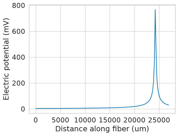
Let’s simulate a recording electrode directly over this end of the fiber. We can do this by obtaining the electrical potentials along the fiber in response to a unit stimulus (1 mA) from a point source. By the principle of reciprocity, we can then use these potentials to calculate the voltage generated at the recording site by each fiber segment’s transmembrane currents.

x = 0
y = 100  # place electrode 100 um above the fiber
z = 0.9 * fiber.length  # place electrode 90% along the fiber
current = 1  # mA, unit stimulus
sigma = 1  # S/m, extracellular conductivity

# calculate the potentials generated by a point source at the electrode location
recording_potentials = fiber.point_source_potentials(x, y, z, current, sigma)
plt.figure()
plt.plot(fiber.longitudinal_coordinates, recording_potentials)
plt.xlabel('Distance along fiber (um)')
plt.ylabel('Electric potential (mV)')
plt.show()

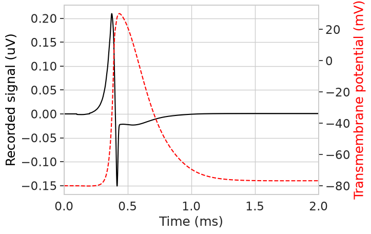
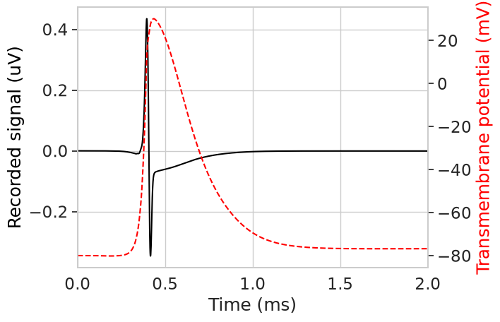
Now we can obtain the signal recorded by the electrode using record_sfap() method.

downsample = 1  # factor by which to downsample recording time
sfap, downsampled_time = fiber.record_sfap(
    recording_potentials, downsample=downsample
)  # record the single fiber action potential

plt.figure()
plt.plot(downsampled_time, sfap, color='black')
plt.xlim(0, 2)
plt.xlabel('Time (ms)')
plt.ylabel('Recorded signal (uV)', color='black')
# plot transmembrane voltage on second axis
plt.twinx()
plt.gca().yaxis.grid(False)
plt.plot(
    stimulation.time, list(fiber.vm[fiber.loc_index(0.9)]), color='red', linestyle='--'
)
plt.ylabel('Transmembrane potential (mV)', color='red')
plt.show()

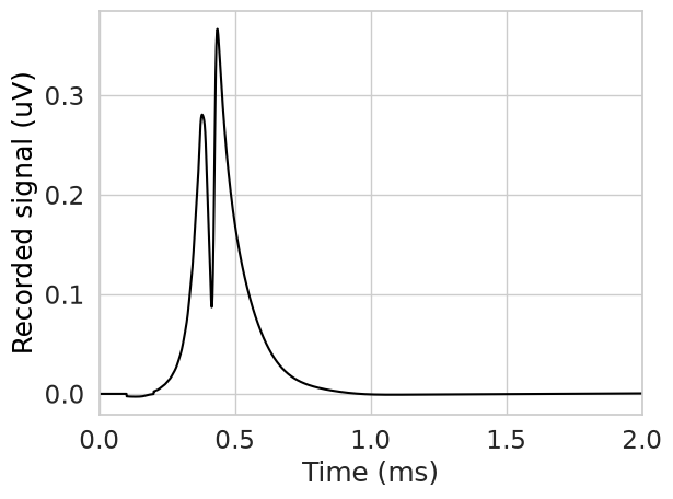
The process can be repeated for a multipolar recording setup. Let’s try bipolar recording.

rec_potentials = np.zeros(len(fiber.sections))
for loc, weight in zip([0.89, 0.91], [-1, 1]):
    rec_potentials += (
        fiber.point_source_potentials(x, y, loc * fiber.length, current, sigma) * weight
    )
sfap, downsampled_time = fiber.record_sfap(
    rec_potentials, downsample=downsample
)  # record the single fiber action potential

plt.figure()
plt.plot(np.array(stimulation.time)[::downsample], sfap, color='black')
plt.xlim(0, 2)
plt.xlabel('Time (ms)')
plt.ylabel('Recorded signal (uV)', color='black')
# plot transmembrane voltage on second axis
plt.twinx()
plt.plot(
    stimulation.time, list(fiber.vm[fiber.loc_index(0.9)]), color='red', linestyle='--'
)
plt.ylabel('Transmembrane potential (mV)', color='red')
plt.gca().yaxis.grid(False)
plt.show()

You could also record the activity of many fibers, and then sum the signals to obtain the compound action potential. Notice that the compound action potential is greater in magnitude, since the signals sum. Note that you can modify fiber positioning with the fiber.set_xyz() function. For now we’ll leave the fiber locations as is.

fibers = [
    build_fiber(FiberModel.MRG_INTERPOLATION, diameter=d, n_nodes=n_nodes)
    for d in [8, 9, 10]
]
sfaps = []
for fib in fibers:
    fib.record_im(allsec=True)
    fib.record_vext()
    fib.potentials = fib.point_source_potentials(0, 250, fib.length / 2, 1, 10)
    stimulation.run_sim(-1.5, fib)
    recording_potentials = fib.point_source_potentials(x, y, z, current, sigma)
    sfaps.append(fib.record_sfap(recording_potentials, downsample=downsample)[0])

Running: -1.5
	N aps: 1, time 0.385
Running: -1.5
	N aps: 1, time 0.383
Running: -1.5
	N aps: 1, time 0.379

sfap = np.sum(sfaps, axis=0)

plt.figure()
plt.plot(np.array(stimulation.time)[::downsample], sfap, color='black')
plt.xlim(0, 2)
plt.xlabel('Time (ms)')
plt.ylabel('Recorded signal (uV)', color='black')
plt.show()

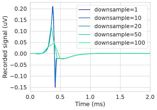
The downsample parameter can be used to reduce the timesteps processed during SFAP calculation. This can reduce memory and computation time for sfaps, but can compromise the accuracy of the signal.

plt.figure()
downsamples = [1, 10, 20, 50, 100]
colors = plt.cm.winter(np.linspace(0, 1, len(downsamples)))
fiber = fibers[2]
for i, downsample in enumerate(downsamples):
    recording_potentials = fiber.point_source_potentials(x, y, z, current, sigma)
    sfap, downsampled_time = fiber.record_sfap(
        recording_potentials, downsample=downsample
    )
    plt.plot(downsampled_time, sfap, label=f'downsample={downsample}', color=colors[i])
plt.xlim(0, 2)
plt.xlabel('Time (ms)')
plt.ylabel('Recorded signal (uV)')
plt.legend()

<matplotlib.legend.Legend at 0x7fa405d16f50>